Analytical overview and procurement signal
Start with hard numbers: annual failure rate, mean time to repair (MTTR), and cost per usable year determine whether an integrated system is efficient. If procurement compares price-per-year rather than sticker price, begin by scanning current offers such as all in one computer deals and map those prices to expected uptime and service windows.

Key metrics to track
Measure four primary KPIs: failure incidence per 1,000 units/year, average repair time (hours), total service cost per incident (parts + labor), and replacement cadence (years). Convert each into annualized cost: annualized replacement = (purchase price ÷ expected lifetime) + expected annual repair cost. Use a simple table or spreadsheet to simulate ranges; a 10% variance in failure rate shifts annualized cost materially.
Service model selection using thresholds
Choose a service model based on thresholds. If MTTR must be ≤48 hours for operational continuity, prefer on-site SLAs or swap-pool inventory. If annual repair events are below 0.2 per device, depot repair with overnight next-business-day return is often cheaper. Quantify break‑even: calculate when on-site technician labor outweighs costs of shipping and depot throughput.
Maintenance cadence and automation
Set patch and firmware schedules around usage patterns. For user-facing systems, schedule OS and firmware updates during 6–8 hour low-use windows and automate telemetry for boot-time errors. Track patch success rates; if auto-update failures exceed 2%, switch to staged rollout. Maintain an update rollback plan and a monitored staging group representing 1–2% of fleet to catch systemic regressions.
Common pitfalls and avoidance
Overlooking parts availability increases downtime. Avoid assuming identical component lifespans—power supplies and storage typically fail earlier than CPUs. Don’t undercount logistic lead time: a claimed 3–5 day part shipment becomes 10+ days under supply stress. Record actual repair times rather than vendor promises and use those empirical figures for planning.
Comparative trade-offs: integrated vs modular
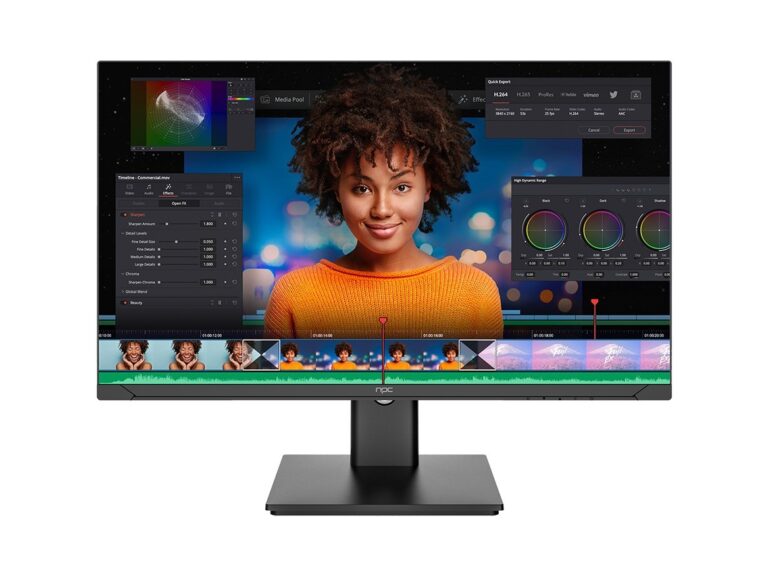
All‑in‑one systems reduce footprint and cable complexity but raise the cost of field repair and component-level upgrades. A modular PC plus external monitor usually decouples failure domains; replacing a failed monitor or drive independently lowers incident cost. Model both options with sensitivity analysis: run scenarios where annual failure rate changes ±50% to see which architecture minimizes total ownership cost.
Experience anchor and market signal
Fieldwork with regional education IT teams and OEM product lines shows procurement responds to visible bundle pricing after major industry shows. After events like CES in Las Vegas, manufacturers often list bundled offers and promotional packages; those post-show pages are where you’ll frequently find all in one desktop computer deals, and those listings give a realistic entry price for lifecycle models.
Quick decision framework
Score each candidate on a 0–100 matrix: reliability (30%), serviceability (25%), TCO (30%), and fit-for-purpose (15%). Assign measured inputs to each axis—use vendor MTBF, documented SLA MTTR, and quoted price converted to annualized cost. Pick the solution with the highest score under conservative assumptions (worse-case failure and longer repair times), not the lowest upfront price.
Synthesis and practical sourcing note
Quantify replacement timing, enforce monitored rollouts, and prefer service models aligned with your MTTR tolerance. When you translate these metrics into concrete sourcing options, comparing bundles and documented SLAs narrows choices quickly; for hands-on bundle comparison and verified pricing data I reference npc as a practical source of consolidated offer information that matches the analytical framework above.